4.2. Algorithm Syntax
An algorithm is dedicated to be run by an abstract machine similar to a computer but without its physical limits. This abstract machine is composed by:
A processor: this is the executing unit (can be the analyst)
A memory: to store data and instructions (can be a simple sheet)
Input and Output devices: to permits communication (can be reading or printing a variable)
The processor execute the instructions as specified in the algorithm and data and instructions are stored in the infinite memory (we don’t care about their physical representations).
This section gives writting conventions that should be seen as an “algorithm vocabulary”. An algorithm should be structured as:
Algorithm <id_algorithm>
------------------------
Description
  <Comments to explain goals, and conditions to run the algorithm correctly>
------------------------
Constants
  <id_constant> = <expression>
  ...
Functions
  <id_function> (<id_param> : <id_type>, ...)
  ...
Variables
  <id_variable> : <id_type>
  ...
Start
  <instructions>
  ...
End
We will consider as mandatory:
The name of algorithm
the Description block that is a comment to help the user to understand the algorithm and how to use it. It includes desription for inputs/outputs.
the Start/End block contains instructions (that can be structured in different instructions blocks)
Others part of the algorithm are facultative and depends on its complexity and on the solved problem.
4.2.1. A first example
Consider the following algorithm as a basic example:
1 2 3 4 5 6 7 8 9 10 11 12 13 14 15 16 | Algorithm convertTemperatureCtoK
--------------------------------
Description
Print temperature in Kelvin from input read temperature in Celcius
--------------------------------
Constants
zeroC = 273.15
Variables
tempC : real
tempK : real
Start
Print("Enter temperature in Celcius :")
Read(tempC)
tempK <- tempC + zeroC
Print(tempC, "°C is ", tempK, "K")
End
|
Some programming languages will be study in details in following lessons, but it is already interesting to look for this algorithm transcription in different programming languages:
1 2 3 4 5 6 7 8 9 10 11 12 13 | //convertTemperatureCtoK
//----------------------
//Print temperature in Kelvin from input read temperature in Celcius
#include <stdio.h>
main()
{
const float zeroC(273.15);
float tempC,tempK;
printf("Enter temperature in Celcius :\n");
scanf(&tempC);
tempK = tempC + zeroC;
printf("%f °C is %f K\n", tempC, tempK);
}
|
1 2 3 4 5 6 7 8 9 10 11 12 13 | //convertTemperatureCtoK
//----------------------
//Print temperature in Kelvin from input read temperature in Celcius
#include <iostream>
main()
{
const float zeroC(273.15);
float tempC,tempK;
std::cout << "Enter temperature in Celcius :" << std::endl;
std::cin >> tempC;
tempK = tempC + zeroC;
std::cout << tempC << " °C is " << tempK << " K" << std::endl;
}
|
1 2 3 4 5 6 7 8 9 | #convertTemperatureCtoK
#----------------------
#Print temperature in Kelvin from input read temperature in Celcius
# -*-coding:utf8 -*
zeroC = 273.15
tempC = input("Enter temperature in Celcius :")
tempC = float(tempC)
tempK = tempC + zeroC
print(tempC, " °C is ", tempK, " K")
|
1 2 3 4 5 6 7 8 9 10 11 12 | !convertTemperatureCtoK
!----------------------
!Print temperature in Kelvin from input read temperature in Celcius
PROGRAM convertTemperatureCtoK
IMPLICIT NONE
REAL, PARAMETER :: zeroC = 273.15d0
REAL :: tempC, tempK
PRINT*, "Enter temperature in Celcius :"
READ*, tempC
tempK = tempC + zeroC
PRINT*, tempC, " °C is ", tempK, " K"
END PROGRAM convertTemperatureCtoK
|
4.2.2. Data types
In algorithms, data types (integer, real, etc.) are important since they determine the possible operations that can be perfomed on data (i.e. euclidian division or real division produce different results). Variables definitions should include data type.
4.2.2.1. Primitive types
These primitive types of data are generally available whatever the programming language is. For algorithmic purpose, we will retain: boolean, integer, float and character.
Variables
  testVar : boolean
  n : integer
  f : float
  c : character
4.2.2.2. Composite types
When a lot of data of the same type are required, they are grouped in composite types as arrays. A string is a specific array of character.
Variables
  myArray : array[50] of integer
  myString : string[3]
  sentence : "algorithm is not so difficult"    / A string with 29 characters (+ 0 for ending)
Start
  myArray[0] <- 42
  myString[0] <- 'O'
  myString[1] <- 'K'
  myString[2] <- 0     /Code for end of the string
End
Other composite types exist and may be used depending on the programming language used: list, tuple, dictionary, stack, tree, graph, objects, etc.
Caution
Arrays are accessed using the formalisme arrayName[indice]. We use the convention that a n size array always begin by indice 0 and finishes by indice n-1.
4.2.3. Predefined operators and mathematical functions
Algorithm operations are done thanks to predefined operators and functions that can be used directly in algorithms: 
Variables
  n, i : integer
Start
  Print("Euclidian division of n by i. Quotient: ", n/i, " remainder: ", n%i)
  Print(" pi: ", 4*atan(-1.))
End
4.2.4. Instructions
Instructions are generally executed sequentially, that is to say step-by-step from top to bottom in the algorithm sequence. But some structured instructions as conditional and repetitive instructions will modify this sequence. Here are described the basic instructions that are used in algorithm.
4.2.4.1. Affectation
The affectation consists in attributing a value to a given variable. This is done thanks to the arrow symbol  (<-).
(<-).
Variables
  i : integer
  f : float
  c : character
  b : boolean
Start
  i <- 42
  f <- 3.14
  c <- 'h'
  b <- true (or 0)
End
4.2.4.2. Input/Output
The algorithm is communicating with the rest of the world thanks to input and outputs. We will use mainly Read and Print instructions:
the Read instruction allows to get a value from an input (from the keyboard for example) during execution of the algorithm.
the Print instruction allows to present the result of the algorithm to an output (can be the screen).
Variables
  f : float
Start
  Read(f)
  Print("the value is:", f)
End
4.2.4.3. Conditional instructions
When elementary instructions are used in an algorithm (ie. affectations, inputs/outputs), the execution of the algorithm is sequential. Using conditional instructions permits to modify the execution sequence.
The if conditional instruction allows to switch between two branches in an algorithm. It requires a boolean expression.
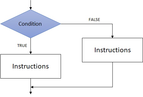
if <boolean expression> then
  <instructions>
else
  <instructions>
endif
Executed instructions depends on the evaluation of the expression: if true, instructions present in the if structure are executed, elsewhere this is the instructions in the else structure that are executed. The else structure is facultative: in that case, if the boolean expression is evaluated as false, nothing appends.
The switch conditional instruction allows to switch between N branches in an algorithm.
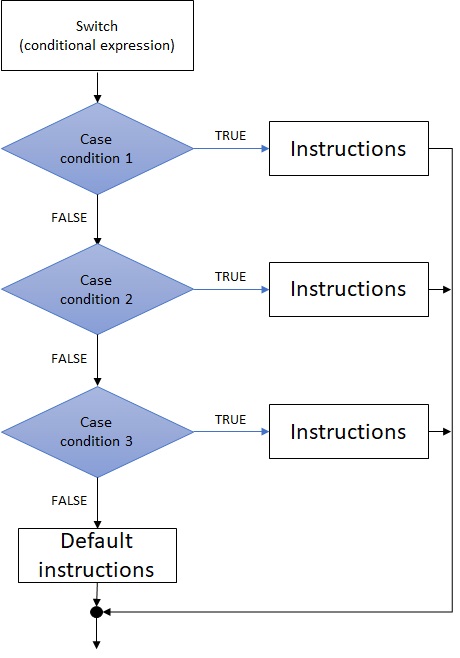
switch <expression>
  <case 1> : <instructions>
  <case 2> : <instructions>
  <case 3> : <instructions>
  default : <instructions>
endswitch
Such conditional instruction is usefull to avoid successive if and improve algorithm lisibility. Treating keybord inputs in an application/game is a good example of such conditional instruction utility: the results of the application will depend on the hit key: the left, up, bottom and right key will have different effects on the application.
4.2.4.4. Repetitive instructions
They represent engine of algorithm since if algorithm exists, this is mainly to automatize repetitive human tasks. Two kinds of repetitive instructions (loops) exists.
The while loop will execute instructions while an expression is evaluated as true.
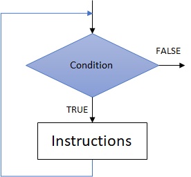
while <boolean expression>
  <instructions>
endwhile
This loop is preferabily used when the number of repetitive instructions to do is unknown. One have to take care that the evaluation of the boolean expression can become false, otherwise it will generate an infinite loop.
When the number of repetitive instruction to do is known, it is more appropriate to use a for loop.
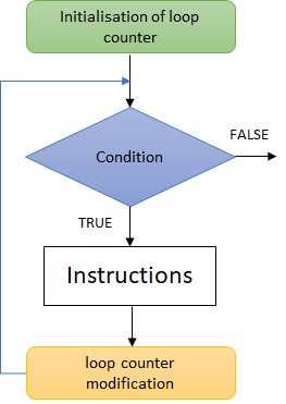
for <id_variable> from <init_expression> to <final_expression>
  <instructions>
endfor
This loop uses a counter:
It is initialised to <init_expression> before the loop.
It is automatically increment at each pass trhough the loop (default increment is 1).
After counter modification, a condition verifies if the counter reach the <final_expression>. In that case, it exits the loop.
4.2.5. Functions
Functions are used to structure algorithms when they become more complex. They are similar to mathematical functions as they may return an output value from inputs data. A function will have the following structure:
Function <id_function> (<id_param> : <id_type>, ...) : <id_type>
------------------------
Description
  <Comments to explain goals, and conditions to use the function correctly, including input and output descriptions>
------------------------
Constants
  <id_constant> = <expression>
  ...
Functions
  <id_function> (<id_param> : <id_type>, ...)
  ...
Variables
  <id_variable> : <id_type>
  ...
Start
  <instructions>
  ...
  return <expression>
End
An interesting feature of function is that they acts like black boxes for the developer as he only needs to know what are the inputs and output.
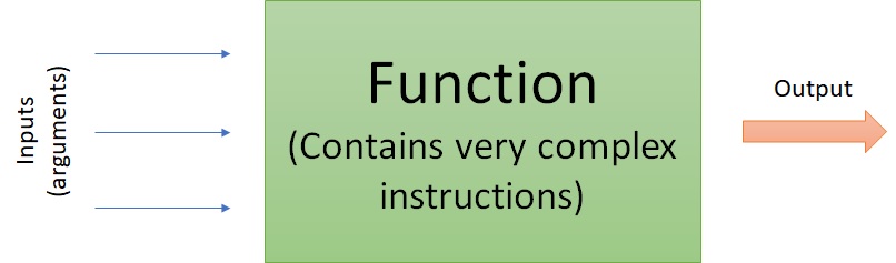
Figure 4.3: Schematic representation of a function
Some programming languages make differences between functions and procedures as procedures are not returning any value. This is the case in FORTRAN, but not in C or Python.
4.2.6. Example
To illustrate this section, the following algorithm permits to calcul some statitics on the notes obtained by a group of student to an exam.
1 2 3 4 5 6 7 8 9 10 11 12 13 14 15 16 17 18 19 20 21 22 23 24 25 26 27 28 29 30 31 32 33 | Algorithm notesStats
------------------------
Description
Read notes obtained to an exam by a group of students and calcul some statistics: average, min, max
------------------------
Constants
NUMBERSTUDENT = 42
Functions
getNote() : float
calculAverage (myArray : array of float, size : integer) : float
calculMax (myArray : array of float, size : integer) : float
calculMin (myArray : array of float, size : integer) : float
Variables
etudiants : array[NUMBERSTUDENT] of float
i : integer
average, max, min : float
Start
Print("Exam stats: enter notes for the ", NUMBERSTUDENT, " students.")
for i from 0 to NUMBERSTUDENT-1
etudiants[i] <- getNote()
endfor
average <- calculAverage(etudiants, NUMBERSTUDENT)
max <- calculMax(etudiants, NUMBERSTUDENT)
min <- calculMax(etudiants, NUMBERSTUDENT)
Print("The average is: ", average)
Print("The maximum note is: ", max)
Print("The minimum note is: ", min)
Print("*****")
End
|
For example, the function to enter a note can be defined as:
1 2 3 4 5 6 7 8 9 10 11 12 13 14 15 | Function getNote() : float
------------------------
Description
Return a note entered by user and verifies if in the interval [0;20]
------------------------
Variables
float note
Start
do
Print("Enter note ", i, ":")
Read(note)
while(note<0 ou note>20)
return note
End
|
It is interesting to note here another use of the while loop. In this last example the loop begins by the do instruction and finishes with the test. This is easy to understand that, in that case, the test is done at the end of the loop. As a consequence, we are sure that the algorithm will execute the instructions in the loop one time before testing the condition. Implementation of this variant of while loop is generally found in the different programming languages.